MESS Machine Learning (ML) Inference
Once you have performed a sufficient number of simulations you can now use these simulations to perform community assembly model selection and parameter estimation for observed community data. In this short tutorial we will demonstrate the fundamentals of how this works.
The MESS.inference architecture is based on the powerful and
extensive scikit-learn python machine
learning library. Another really amazing resource I highly recommend is
the Python Data Science Handbook.
- Download and examine example empirical data
- Fetch pre-baked simulations
- Supported ensemble methods
- ML assembly model classification
- ML parameter estimation
- Perform posterior predictive simulations
- Experiment with other example datasets
- References
Download and examine example empirical data
We will be using as an example dataset of community-scale COI sequences (~500bp) and densely sampled abundances for the spider community on the island of La Reunion, an overseas department of France, and the largest of the Mascarene islands, located in the Indian Ocean approximately 1000 km from Madagascar. The data we will be using was collected and published by Emerson et al (2017). For this exercise, we will use the pre-processed summary statistics which were generated from the real data and which are available in the MESS github repository. For further instruction on properly formatting and converting raw data into MESS-ready format see the MESS raw data handling page.
In a new cell in your notebook you can download the Reunion spider data like this:
!wget https://raw.githubusercontent.com/messDiv/MESS/master/empirical_data/Reunion_spiders/spider.dat
NB: The!prior to the command here indicates that the jupyter notebook should interpret this as a bash command executed at the command line. This is a handy way of executing bash commands from within the notebook environment, rather than returning to a terminal window on the cluster. It’s just a nice shortcut.
Now make a new cell and import MESS and pandas (which is a python structured data library providing the DataFrame class), and read in the data you just downloaded.
%matplotlib inline
import MESS
import pandas as pd
spider_df = pd.read_csv("spider.dat", index_col=0)
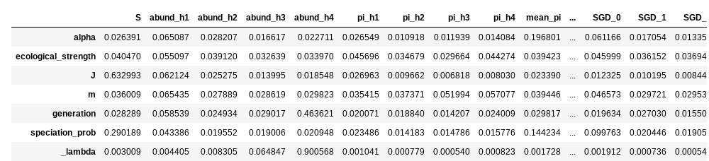
spider_df[:5]
Special Note: The
%matplotlib inlinecommand tells jupyter to draw the figures actually inside your notebook environment. If you don’t include this your figures won’t show up!NB: Importing pandas as
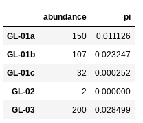
pdis pretty cannonical. It makes typing out pandas commands shorter because you can reference it aspdrather thanpandas.NB: The final line in the above command asks python to display the first 5 rows of the
spider_dfdataframe. It should look like this:
Fetch pre-baked simulations
Since it can take quite some time to run a number of simulations
sufficient for model selection and parameter estimation we will use a
suite of pre-baked simulations generated ahead of time. This dataset is
composed of ~8k simulations under each of the community assembly models with
a few of the parameters sampled from distributions and the rest set to fixed
values. Fetch this dataset from the compphylo site with wget:
!wget https://compphylo.github.io/Oslo2019/MESS_files/MESS_simulations/SIMOUT.txt
!wc -l SIMOUT.txt
100%[======================================>] 14,234,338  50.0M/s   in 0.3s
2019-08-11 01:25:27 (50.0 MB/s) - "SIMOUT.txt" saved [14234338/14234338]
24440 SIMOUT.txt
NB: Thewccommand counts the number of lines if you pass it the-lflag. You can see this series of ~25k simulations is about 14MB.
Supported ensemble methods
MESS currently supports three different scikit-learn ensemble methods for
classification and parameter estimation:
- RandomForest (rf):
- GradientBoosting (gb):
- AdaBoost (ab):
ML assembly model classification
The first step is now to assess the model of community assembly that
best fits the data. The three models are neutral, in which all
individuals are ecologically equivalent; competition, in which
species have traits, and differential survival probability is weighted
by distance of traits from the trait mean in the local community (closer
to the trait mean == higher probability of death); and filtering, in
which there is an environmental optimum, and proximity of trait values
to this optimum is positively correlated with survival probability.
Basically we want to know, are individuals in the local community ecologically equivalent, and if not are, they interacting more with each other or more with the local environment.
Here we create a MESS.inference.Classifier object and pass in the
empirical dataframe, the simulations, and specify RandomForest (rf) as
the algorithm to use (other options are GradientBoosting (gb) and
AdaBoost (ab)). Full documentation of all the machine learning inference
architecture is available in the MESS API specification.
cla = MESS.inference.Classifier(empirical_df=spider_df, simfile="SIMOUT.txt", algorithm="rf")
est, proba = cla.predict(select_features=False, param_search=False, quick=True, verbose=True)
The Classifier.predict() method provides a sophisticated suite
of routines for automating machine learning performance tuning. Here we
disable all of this in order for it to run quickly, trading
accuracy for performance. The select_features argument controls
whether or not to prune summary statistics based on correlation and
informativeness. The param_search argument controls whether or not
to exhaustively search the space of parameters to maximize accuracy of
the ML algorithm selected. Finally, the quick argument subsets the
size of the simulation database to 1000 simulations, again as a means of
running quickly to verify, for example, whether all the input data and
simulations are formatted properly. In normal conditions, when you
want to investigate real data you should use select_featers=True,
param_search=True, quick=False. This will result in much more accurate
inference, yet will take much more time to run.
The call to cla.predict() returns both the most likely community
assembly model (est) and the model probabilities (proba), which
you can view:
from IPython.display import display
display(est, proba)
NB: The first line of this codeblock imports thedisplaymethod from theIPythonlibrary, which makes pd.DataFrames display nicely.
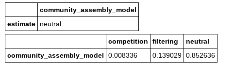
Here we see that the neutral model is vastly favored over the
competition and fitering models.
Now we can examine the weight of importance of each feature, an
indication of the contribution of each summary statistic to the
inference of the ML algorithm. You can also get a quick and dirty plot
of feature importances directly from the Classifier object with the
plot_feature_importances() method.
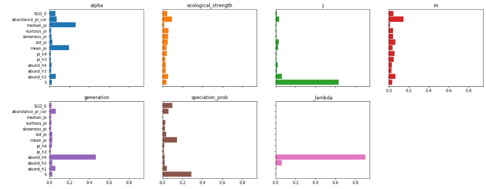
display(cla.feature_importances())
cla.plot_feature_importance(figsize=(5,5))
NB: Thefigsizeargument controls the size of the output figure. The default is(10, 10), so here we just make it a bit smaller to fit better in the notebook window.
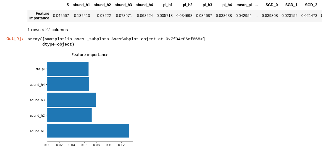
The plot_feature_importance() method prunes out all the summary
statistics that contribute less than 5% of information to the final
model. This method is simply for visualization. Here you can see that
the shape of the abundance distributions (as quantified by the first 4
Hill numbers) and the standard deviation of nucleotide diversity (pi)
within the local community are the most important summary statistics for
differentiating between the different community assembly models.
ML parameter estimation
Now that we have identified the neutral model as the most probable, we can estimate parameters of the emipirical data given this model. Essentially, we are asking the question “What are the parameters of the model that generate summary statistics most similar to those of the empirical data?”
The MESS.inference module provides the Regressor class, which
has a very similar API to the Classifier. We create a Regressor
and pass in the empirical data, the simulations, and the machine
learning algorithm to use, but this time we also add the
target_model which prunes the simulations to include only those of
the community assembly model of interest. Again, we call predict()
on the regressor and pass in all the arguments to make it run fast, but
do a bad job.
rgr = MESS.inference.Regressor(empirical_df=spider_df, simfile="SIMOUT.txt", target_model="neutral", algorithm="rfq")
est = rgr.predict(select_features=False, param_search=False, quick=True, verbose=False)
NB: Note that here we ask for therfqalgorithm, which designates random forest quantile regression, and allows for constructing prediction intervals, something the stockrfalgorithm doesn’t do. The gradient boosting method (gb) provides prediction intervals natively.
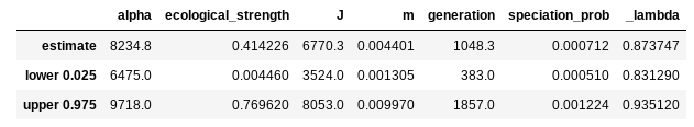
The return value est is a dataframe that contains predicted values
for each model parameter and 95% prediction intervals, which are
conceptually in the same ball park as maximum likelihood confidence intervals
(CI) and and Bayesian highest posterior densities (HPD).
display(est)
Similar to the classifier, you can also extract feature importances from the regressor, to get an idea about how each feature is contributing to parameter estimation. In this case, the feature importance plots are a little more useful than the giant table. Also note that we’re requesting a slighly larger figure, because this time there will be much more information.
display(rgr.feature_importances())
rgr.plot_feature_importance(figsize=(20,8))
You can see that some parameters are strongly driven by one or a couple
of features, and for some the feature importances are more diffuse. For
example species richness (S) contributes overwhelmingly to
estimation of local community size (J), which makes sense. On the
other hand, many more factors seem to contribute equally to estimation
of migration rate (m).
Perform posterior predictive simulations
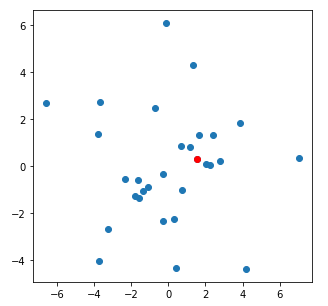
Finally, a very important step in machine learning inference is to validate the parameter estimates by performing posterior predictive checks (PPCs). The logic of this procedure is that we will generate a suite of simulations using our most probable parameter estimates, and compare these simulations to our empirical data. For our purposes here we will project the summary statistics of observed and simulated datasets into principle component space. If the parameter estimates are a good fit to the data then our posterior predictive simulations will cluster together with the real data, whereas if the parameter estimates are a poor fit, then the real data will be quite different from the simulations.
Spoiler alert: Posterior predictive simulations can take quite a while to run. With the parameters we get even with this toy data a reasonable number of sims could take a couple hours. So! For the purpose of this exercise we are going to transform the estimated parameters to make the simulations run faster. DO NOT DO THIS WITH YOUR REAL DATA!
est["J"] /= 2
est["m"] *= 10
est["_lambda"] /= 2
est
Here we reduced the size of the local community (J), increased the
rate of migration (m), and decreased the duration of the simulation
(_lambda). All these things will make the simulations run more
quickly. Now go ahead and run this next cell, it should take one to two
minutes.
MESS.inference.posterior_predictive_check(empirical_df=spider_df,
                                          parameter_estimates=est,
                                          est_only=True,
                                          nsims=20,
                                          verbose=True,
                                          force=True)
  Generating 20 simulation(s).
[####################] 100%  Finished 19 simulations   | 0:02:57 |

  Calculating PCs and plotting
NB: Theposterior_predictive_check()function can also accept anipyclientparameter to specify to use an ipyparallel backend. For simplicity here we will not use this option, but in reality it would be a good idea to parallelize the posterior predictive simulations. See the MESS parallelization docs for more info about how to implement the parallel backend.
This time the only thing we have to pass in is the empirical data and
the dataframe of prediction values, but we show a couple more arguments
here for the sake of completeness. Setting est_only to True will use
only the exact parameter estimates for all simulations, whereas setting it to
False will sample uniformly between the upper and lower prediction interval
for each simulation. nsims should be obvious, the number of posterior
predictive simulations to perform. force will overwrite any pre-existing
simulations, thus preventing mixing apples with oranges from different
simulation runs. On the other hand if this is False (the default), then
this is a handy way to add more PPCs to your analysis.
The posterior_predictive_check() method will also display the summary
statistics for the simulated and observed data projected into PC space. The
observed data is colored in red. Here is a pretty typical example of a good
fit of parameters to the data:
And here is a nice example of a poor fit of parameters to the data:
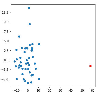
Quite a striking, and obvious difference.
Experiment with other example datasets
Now you may wish to experiment with some of the other empirical datasets which are provided on the MESS github repo, or with exploring the substantial MESS inference procedure API documentation where we show a ton of other cool stuff MESS is capable of that we just don’t have time to go over in this short tutorial.
References
Emerson, B. C., Casquet, J., López, H., Cardoso, P., Borges, P. A.,
    Mollaret, N., … & Thébaud, C. (2017). A combined field survey and
    molecular identification protocol for comparing forest arthropod
    biodiversity across spatial scales. Molecular ecology resources, 17(4),
    694-707.