MESS Model Parameters
The parameters contained in a params file affect the behavior of various parts of the forward-time and backward-time assembly process. The defaults that we chose are fairly reasonable values as as starting point, however, you will always need to modify at least a few of them (for example, to indicate the location of your data), and often times you will want to modify many of the parameters.
Below is an explanation of each parameter setting, the eco-evolutionary process that it affects, and example entries for the parameter into a params.txt file.
NB: Most parameters for which is it sensible to do so will accept a prior range which will be sampled from uniformly for each simulation (e.g. a value of1000-5000for parameterJwill choose a newJfor each simulation inclusively bounded by these values).
simulation_name
The simulation name is used as the prefix for all output files. It should be a unique identifier for this particular set of simulations, meaning the set of parameters you are using for the current data set. When I run multiple related simulations I usually use names indicating the specific parameter combinations (e.g., filtering_nospeciation, J5000_neutral).
Example: New community simulations are created with the -n options to MESS:
## create a new assembly named J1000_neutral
$ MESS -n J1000_neutral
project_dir
A project directory can be used to group together multiple related simulations. A new directory will be created at the given path if it does not already exist. A good name for project_dir will generally be the name of the community/system being studied. The project dir path should generally not be changed after simulations/analysis are initiated, unless the entire directory is moved to a different location/machine.
Example entries into params.txt:
/home/watdo/MESS/galapagos         ## [1] create/use project dir called galapagos
galapagos                          ## [1] create/use project dir called galapagos in cwd (./)
generations
This parameter specifies the amount of time to run forward-time simulations. It can be specified in a number of different ways, but overall time can be considered either in terms of Wright-Fisher (WF) generations or in terms of Lambda. For WF generations you should specify an integer value (or a range of integer values) which will run the forward-time process for WF * J / 2 time-steps (where a time-step is one birth/death/colonization/speciation event). For Lambda you may select either an exact Lambda value (a real value between 0 and 1 exclusive), or you can set generations equal to 0, which will draw random Lambda values between 0 and 1 for each simulation.
Example entries into params.txt:
0                   ## [2] [generations]: Sample random Lambda values for each simulation
100                 ## [2] [generations]: Run each simulation for 100 WF generations
50-100              ## [2] [generations]: Sample uniform between 50-100 WF generations for each simulation
community_assembly_model
With this parameter you may specify a neutral or non-neutral scenario for the forward time process. There are currently three different options for this parameter: neutral, filtering, or competition. The neutral case indicates full ecological equivalence of all species, so all individuals have an equal probability of death at each time-step. In the filtering and competition models survival probability is contingent on proximity of species trait values to the environmental optimum, or distance from the local trait mean, respectively. You may also use the wildcard * here and MESS will randomly sample one community assembly model for each simulation.
Example entries into params.txt:
neutral             ## [3] [community_assembly_model]: Select the neutral process forward-time
filtering           ## [3] [community_assembly_model]: Select the environmental filtering process
*                   ## [3] [community_assembly_model]: Randomly choose one of the community assembly models
speciation_model
Specify a speciation process in the local community. If none then no speciation happens locally. If point_mutation then one individual will instantaneously speciate at rate speciation_prob for each forward-time step. If random_fission then one lineage will randomly split into two lineages at rate speciation_prob with the new lineage receiving n = U~(1, local species abundance) individuals, and the parent lineage receiving 1 - n individuals. protracted will specify a model of protracted speciation, but this is as yet unimplemented.
Example entries into params.txt:
none                ## [4] [speciation_model]: No speciation in the local community
point_mutation      ## [4] [speciation_model]: Point mutation specation process
mutation_rate
Specify the mutation rate for backward-time coalescent simulation of genetic variation. This rate is the per base, per generation probability of a mutation under an infinite sites model.
Example entries into params.txt:
2.2e-08 ## [5] [mutation_rate]: Mutation rate scaled per base per generation
alpha
Scaling factor for transforming number of demes to number of individuals.
alpha can be specified as either a single integer value or as a range
of values.
Example entries to params.txt file:
2000                ## [6] [alpha]: Abundance/Ne scaling factor
1000-10000          ## [6] [alpha]: Abundance/Ne scaling factor
sequence_length
Length of the sequence to simulate in the backward-time process under an infinite sites model. This value should be specified based on the length of the region sequenced for the observed community data in bp.
Example entries to params.txt file:
570 ## [7] [sequence_length]: Length in bases of the sequence to simulate
S_m
S_m specifies the total number of species to simulate in the metacommunity. Larger values will result in more singletons in the local community and reduced rates of multiple-colonization.
Example entries to params.txt file:
500                 ## [0] [S_m]: Number of species in the regional pool
100-1000            ## [0] [S_m]: Number of species in the regional pool
J_m
The total number of individuals in the metacommunity. This value is divided up
among all S_m species following a logseries distribution. J_m values
which are smaller will produce more even abundances in the metacommunity, which
will result in more equal probability of colonization among species.
Example entries to params.txt:
50000               ## [1] [J_m]: Total # of individuals in the regional pool
50000-500000        ## [1] [J_m]: Total # of individuals in the regional pool
speciation_rate
The speciation rate parameter of the birth-death process which generates the metacommunity phylogeny.
Example entries to params.txt:
2 ## [2] [speciation_rate]: Speciation rate of metacommunity
death_proportion
The rate of extinction proportional to the speciation rate for the birth-death metacommunity phylogeny.
Example entries to params.txt:
0.7 ## [3] [death_proportion]: Proportion of speciation rate to be extinction rate
trait_rate_meta
The variance of the Brownian motion process for evolving traits along the metacommunity phylogeny. Smaller values will result in more trait similarity within clades, and larger values will result in more overdispersed traits.
Example entries to params.txt:
2 ## [4] [trait_rate_meta]: Trait evolution rate parameter for metacommunity
ecological_strength
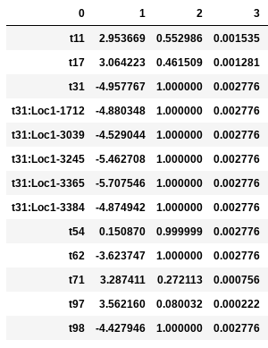
This parameter dictates the strength of interactions in the environmental filtering and competition models. As the value of this parameter approaches zero, ecological strength is reduced and the assembly process increasingly resembles neutrality (ecological equivalence). Larger values increasingly bias probability of death against individuals with traits farther from the environmental optimum (in the filtering model).
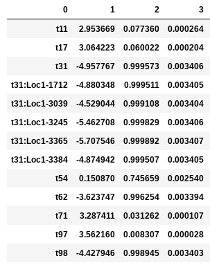
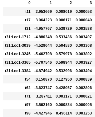
In the following examples the environmental optimum is 3.850979, and the ecological strength is varied from 0.001 to 100. Column 0 is species ID, column 1 is trait value, column 2 is unscaled probability of death, and column 3 is proportional probability of death. Models with strength of 0.001 and 0.01 are essentially neutral. Strength of 0.1 confers a slight advantage to individuals very close to the local optimum (e.g. species ‘t97’).
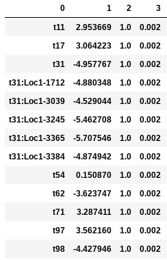
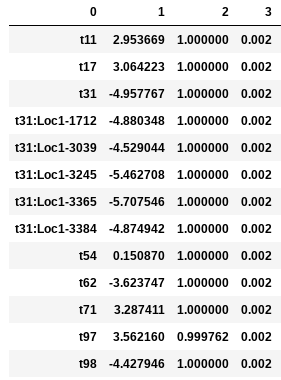
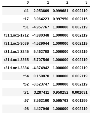
Ecological strength of 1 (below, left panel) is noticeably non-neutral (e.g. ‘t97’ survival probability is 10x greater than average). A value of 10 for this parameter generates a _strong_ non-neutral process (below, center panel: ‘t97’ is 100x less likely to die than average, and the distribution of death probabilities is more varied). Ecological strength values >> 10 are _extreme_ and will probably result in degenerate behavior (e.g. strength of 100 (below, right panel) in which several of the species will be effectively immortal, with survival probability thousands of times better than average).
Example entries to params.txt:
1                  ## [5] [ecological_strength]: Strength of community assembly process on phenotypic change
0.001-1            ## [5] [ecological_strength]: Strength of community assembly process on phenotypic change
name
This is a label for the local community and is used to generate output file names. Generally not that useful unless you’re simulating multiple local communities.
Example entries to params.txt:
island1 ## [0] [name]: Local community name
J
The number of individuals in the local community. This value is fixed for the duration of a community assembly simulation. The size of J will have a strong impact on the consequent species richness and abundance distribution.
Example entries to params.txt:
1000-2000 ## [1] [J]: Number of individuals in the local community
m
The probability at any given timestep that a randomly sampled individual in the local community will be replaced by a migrant from the metacommunity. Larger values of m will generally result in increased species richness.
Example entries to params.txt:
0.01 ## [2] [m]: Migration rate into local community
speciation_prob
Given that a randomly sampled individual from the local community is being replaced by the offspring of another individual from the local community, this parameter defines the probability that this offspring individual will undergo a speciation process.
Example entries to params.txt:
0                  ## [3] [speciation_prob]: Probability of speciation per timestep in local community
0.0001-0.001       ## [3] [speciation_prob]: Probability of speciation per timestep in local community